General Gaussian Models
This page shows examples of conditional knockoffs for the multivariate gaussian models in Section 3.1 of the accompanying paper, which allows for arbitrary mean and covariance matrices.
library("lattice")
library(knockoff)
source('src/knockoff_measure.R')
source('src/util.R')
source('src/cknock_ldg.R')
In this scenario we assume that the distribution of the covariates belongs to a multivariate Gaussian family with unknown mean and unknown covariance matrix. We will separately look at the cases where the number of observations \(n\) is greater than 2 times the dimension \((2p)\) and where \(n<p\) but unlabeled data are available.
Low-Dimensional
We first set up the experiment with \(n>2p\).
set.seed(2019)
# Problem parameters
p = 400         # number of covariates
n = 3*p         # number of observations
k = 60          # number of non-zero regression coefficients
A = 5           # signal amptitude
nonzero = sample(p, k)
beta = 1 * (1:p %in% nonzero) * sample(c(-1,1),p,rep = T)
# Generate the covariates from a multivariate normal distribution
rho = 0.3
Sigma = rho^abs(outer(1:p,1:p,'-'))      # Covariance matrix
Sigma.chol = chol(Sigma)

# Generate the covariates
X = matrix(rnorm(n * p), n) %*% Sigma.chol

# Generate the response from a linear model
Y = X%*%beta*A/sqrt(n) + rnorm(n)
The conditional knockoffs can be generated by calling the function where the method option refers to how \(\mathbf{s}\) is computed and mix is used in the simulations of Section 3.1.2 and discussed in Appendix B.1.1.
Xk.cond = cknockoff.ldg(X,method = 'mix')We can look at the histogram of the original-knockoff correlations for all the \(X_j\) to make sure they are not too high.
cor.ok=diag(cor(X,Xk.cond))
hist(cor.ok,main='',xlab='Original-Knockoff Correlation')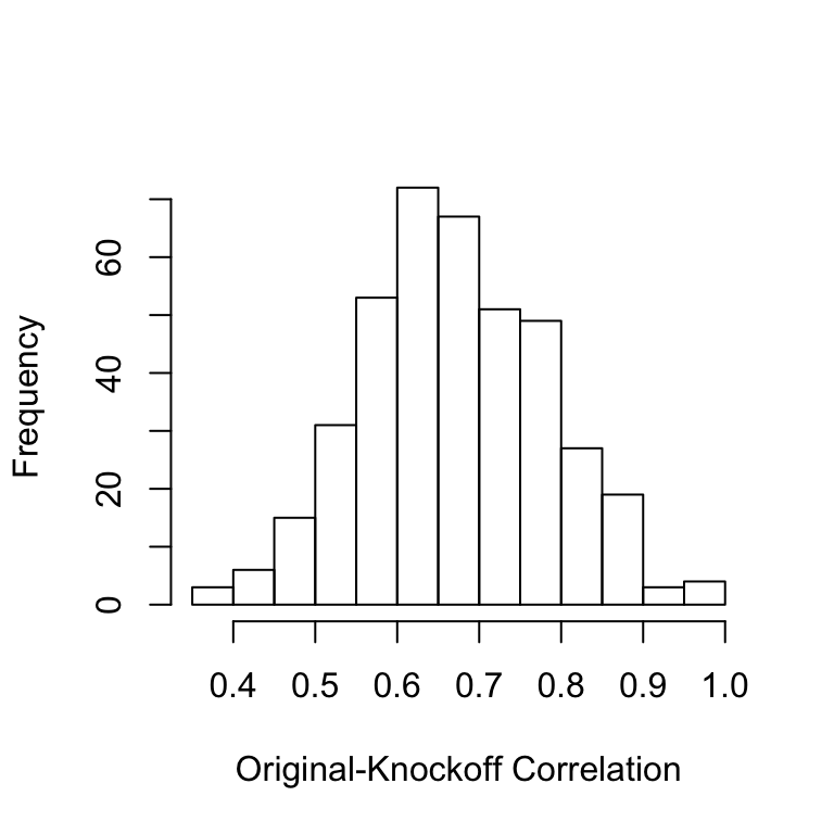
Once we have generated conditional knockoffs, all the usual knockoffs machinery applies.
fdr.level = 0.2
knockoff.stat.fun =  mod.stat.lasso_coefdiff
filter.cond = knockoff.filter(X,Y,
    knockoffs = function(x) {
     Xk.cond
    },
    statistic = knockoff.stat.fun,
    fdr = fdr.level,offset = 1)
# false positive and false negative
c(fp(filter.cond$selected, beta),
 fn(filter.cond$selected, beta))
## [1] 0.1538462 0.9166667As post-diagnostics, we can look at the distribution of the \(W\) statistics.
coloring=rep(1,p); coloring[nonzero]=2 # the color for the true non-zero locations of beta is red
plot(filter.cond$statistic,ylab='Relative Importance Measure (W)',
pch=19,col=coloring,cex=0.5) # plot the statistics used by the knockoff filter
abline(h=filter.cond$threshold,col='blue',lty=3) # indicates the threshold
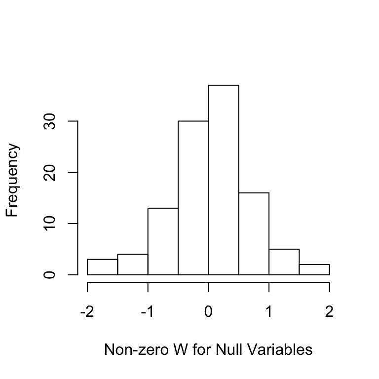
Ws=filter.cond$statistic[-nonzero];Ws=Ws[Ws!=0]
hist(Ws,main='',xlab='Non-zero W for Null Variables')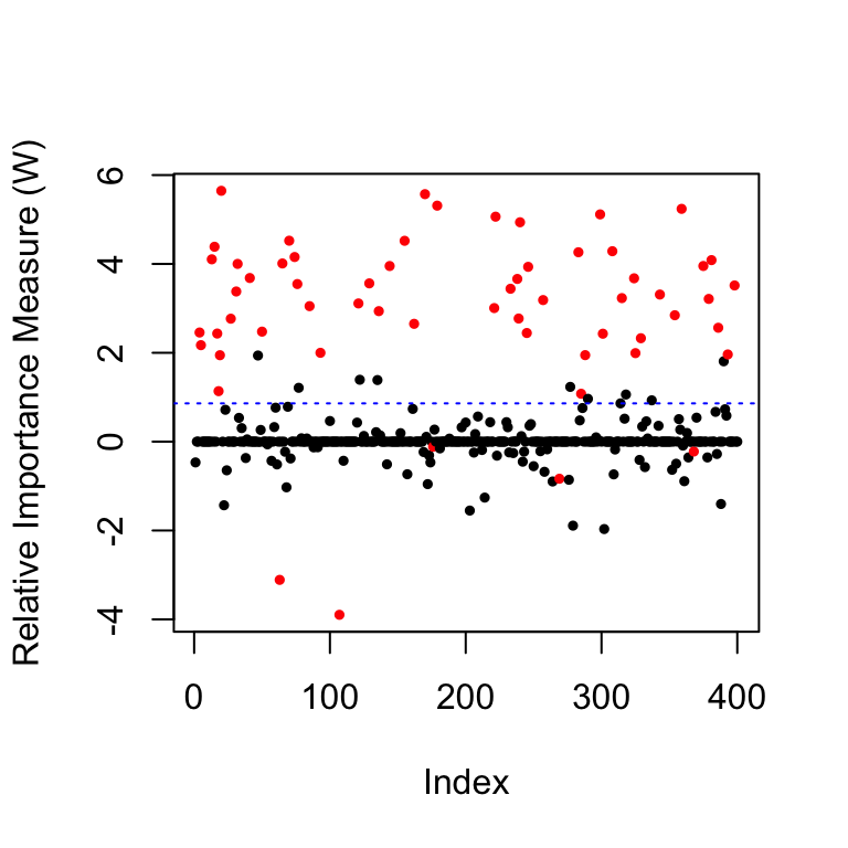
High-Dimensional with Unlabeled Data
In this example, we set up the experiments with a small sample size (\(n<2p\)) but with additional unlabeled data such that the total number of covariate rows is more than \(2p\).
# Problem parameters
n = 300
n.u = 2*p
# Generate labelled and unlabelled covariate
X = matrix(rnorm(n * p), n) %*% Sigma.chol
X.u = matrix(rnorm(n.u * p), n.u) %*% Sigma.chol

# Generate the response from a linear model
Y = X%*%beta*A/sqrt(n) + rnorm(n)
We then generate low-dimensional conditional knockoffs for all the covariates but only keep the rows corresponding to the labeled data.
Xk.star = cknockoff.ldg(rbind(X,X.u),method = 'mix')
Xk.cond = Xk.star[1:n,]
filter.cond = knockoff.filter(X,Y,
knockoffs = function(x) {
Xk.cond
},
statistic = knockoff.stat.fun,
fdr = fdr.level,offset = 1)
# false positive and false negative
c(fp(filter.cond$selected, beta),
fn(filter.cond$selected, beta))## [1] 0.1707317 0.5666667